require(Rdistance)Loading required package: RdistanceLoading required package: unitsudunits database from C:/Users/trent/AppData/Local/R/win-library/4.5/units/share/udunits/udunits2.xmlRdistance (v4.1.1)
This tutorial is a beginner’s guide to doing point transect distance-sampling analysis using Rdistance. Topics covered include input data requirements, fitting a detection function, estimating abundance (or density), and selecting the best fit detection function using AICc. We use the internal datasets thrasherDetectionData and thrasherSiteData (point transect surveys of brown thrashers). This tutorial is current as of version 4.1.1 of Rdistance.
If you haven’t already done so, install the latest version of Rdistance. In the R console, issue install.packages("Rdistance"). After the package is installed, it can be loaded into the current session as follows:
require(Rdistance)Loading required package: RdistanceLoading required package: unitsudunits database from C:/Users/trent/AppData/Local/R/win-library/4.5/units/share/udunits/udunits2.xmlRdistance (v4.1.1)For this tutorial, we use two datasets collected by J. Carlisle on brown thrashers in central Wyoming that are included with Rdistance.
The first dataset, thrasherDetectionData, is a detection data.frame with one row for each detected object. Columns in the data frame are:
siteID = Factor, the site (point) and transect surveyed. Levels are five character codes like ‘TTXPP’ where TT is transect number and PP is the point within the transect.groupsize = Numeric, the number of individuals within the detected group.dist = Numeric, the radial distance from the point to the detected group. Obtain access to the example dataset of thrasher detections and observed distances (thrasherDetectionData) using the following commands:data("thrasherDetectionData")
head(thrasherDetectionData) siteID groupsize dist
1 C1X01 1 11 [m]
2 C1X01 1 183 [m]
3 C1X02 1 58 [m]
4 C1X04 1 89 [m]
5 C1X05 1 83 [m]
6 C1X06 1 95 [m]The second required dataset, thrasherSiteData, is a transect data.frame, with one row for each transect surveyed, and the following required columns:
siteID = Factor, the site (point) and transect surveyed.... = Any additional transect-level covariate columns (these will not be used in this tutorial).Load the example dataset of thrasher transects (thrasherSiteData) using the following commands:
data("thrasherSiteData")
head(thrasherSiteData)
siteID observer bare herb shrub height npoints
1 C1X01 obs5 45.8 19.5 18.7 23.7 1
2 C1X02 obs5 43.4 20.2 20.0 23.6 1
3 C1X03 obs5 44.1 18.8 19.4 23.7 1
4 C1X04 obs5 38.3 22.5 23.5 34.3 1
5 C1X05 obs5 41.5 20.5 20.6 26.8 1
6 C1X06 obs5 43.7 18.6 20.0 23.8 1The final step in data preparation is to make an ‘Rdistance data frame’. ‘Rdistance data frames’ are nested data frames that contain site and detection information in one object. To do this, execute the ‘Rdistance data frame’ constructor function RdistDf, making sure to set pointSurvey to TRUE and specifying which column in thrasherSiteData contains the number of points on each transect.
thrasherDf <- RdistDf(thrasherSiteData
                    , thrasherDetectionData
                    , by = "siteID"
                    , pointSurvey = TRUE
                    , .effortCol = "npoints")
The summary method provides a final check of the data.
summary(thrasherDf, formula = dist ~ groupsize(groupsize))Transect type: point
Effort:
Transects: 120
Total length: 120 [points]
Distances:
0 [m] to 265 [m]: 193
Sightings:
Groups: 193
Individuals: 196 Once the data are imported, the first step is to fit a detection function. Before we do so, explore the distribution of the distances:
hist(unnest(thrasherDf)$dist, n=40, col="grey", main="", xlab="distance (m)")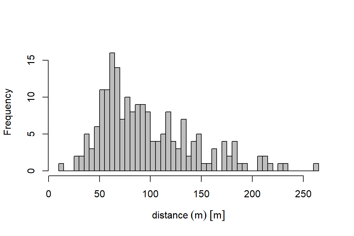
summary(unnest(thrasherDf)$dist) Min. 1st Qu. Median Mean 3rd Qu. Max. NA's
11.00 63.00 86.00 97.16 123.00 265.00 2 Next, we fit a detection function using dfuncEstim to the radial distances collected from the point transects and plot it. We specify the half-normal distance function using option likelihood = "halfnorm". In section 5, we demonstrate an automated process to fit multiple detection functions and compare them using AICc.
dfunc <- dfuncEstim(thrasherDf
                  , formula = dist ~ groupsize(groupsize)
                  , likelihood = "halfnorm")

plot(dfunc)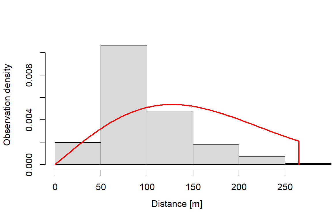
summary(dfunc)Call: dfuncEstim(data = thrasherDf, formula = dist ~
groupsize(groupsize), likelihood = "halfnorm")
Coefficients:
Estimate SE z p(>|z|)
(Intercept) 4.342358 0.03779929 114.8793 0
Message: Success; Asymptotic SE's
Function: HALFNORM
Strip: 0 [m] to 265 [m]
Effective detection radius (EDR): 108.5937 [m]
Probability of detection: 0.1679257
Scaling: g(0 [m]) = 1
Log likelihood: -1004.259
AICc: 2010.54The effective detection radius (EDR) is the essential information from the detection function that will be used to estimate abundance in section 4. The EDR is calculated by integrating the detection function to compute area under the detection function. See the help documentation for EDR for details.
Estimating abundance requires the additional information contained in the the thrasher site dataset, described in section 2, where each row represents one transect. Load the example dataset of surveyed thrasher transects from the package.
We estimate abundance (or density in this case) using abundEstim. If we do not specify a study area size, density is given in the squared units of the distance measurements — in this case, thrashers per square meter. If we set area = 1 hectare (1 ha == 10,000 m^2), both density per square meter and density per hectare will be given. The equation used to calculate the abundance estimate is detailed in the help documentation for abundEstim.
Confidence intervals for abundance are calculated using a bias-corrected bootstrapping method (see abundEstim). Note that, as with all bootstrapping procedures, there may be slight differences in the confidence intervals between runs. Increasing the number of bootstrap iterations (R = 100 used here for brevity) may be necessary to stabilize CI estimates.
# Estimate Abundance - Density; fatalities per m2
fit <- abundEstim(object         = dfunc
                , area           = units::set_units(1, "ha") # density per hectare
                , R              = 100
, ci = 0.95)summary(fit)Call: dfuncEstim(data = thrasherDf, formula = dist ~
groupsize(groupsize), likelihood = "halfnorm")
Coefficients:
Estimate SE z p(>|z|)
(Intercept) 4.342358 0.04513069 96.21741 0
Message: Success; Bootstrap SE's
Function: HALFNORM
Strip: 0 [m] to 265 [m]
Effective detection radius (EDR): 108.5937 [m]
Probability of detection: 0.1679257
Scaling: g(0 [m]) = 1
Log likelihood: -1004.259
AICc: 2010.54
Surveyed Units: 120
Individuals seen: 196 in 193 groups
Average group size: 1.015544
Group size range: 1 to 2
Density in sampled area: 4.408755e-05 [1/m^2]
95% CI: 3.639561e-05 [1/m^2] to 5.312913e-05 [1/m^2]
Abundance in 10000 [m^2] study area: 0.4408755
95% CI: 0.3639561 to 0.5312913The abundance estimate can be extracted from the fit object.
data.frame(fit$estimates) id X.Intercept. density density_lo
1 Original 4.342358 4.408755e-05 [1/m^2] 3.639561e-05 [1/m^2]
density_hi abundance abundance_lo abundance_hi avgEffDistance
1 5.312913e-05 [1/m^2] 0.4408755 0.3639561 0.5312913 108.5937 [m]
avgEffDistance_lo avgEffDistance_hi nGroups nSeen avgGroupSize area
1 100.2841 [m] 117.3683 [m] 193 196 1.015544 10000 [m^2]
surveyedUnits propUnitSurveyed w
1 120 1 265 [m]Fitting several detection functions, choosing the best fitting, and estimating abundance (sections 3 and 4) can be automated using the function autoDistSamp. The function attempts to fit multiple detection functions, uses AICc (by default, but see help documentation for autoDistSamp under criterion for other options) to find the ‘best’ detection function, then proceeds to estimate abundance using the best fit detection function (the distance function with lowest AICc). By default, autoDistSamp tries a large subset of Rdistance’s built-in detection functions, but you can control exactly which detection functions are attempted (see help documentation for autoDistSamp). Specifying plot=TRUE produces a plot of each detection function as it is estimated. Specifying, plot.bs=TRUE plots the selected distance function each iteration of the bootstrap procedure. In this example, we fit the half-normal, hazard rate, exponential, and uniform likelihoods with no expansion terms, we do not plot all fitted functions (plot=FALSE), but we plot the best distance function fitted during each bootstrap iteration.
# Automated Fit - fit several models, choose the best model based on AIC
autoDS <- autoDistSamp(
                     data          = thrasherDf
                   , formula       = dist ~ groupsize(groupsize)
                   , likelihoods   = c("halfnorm", "hazrate", "negexp")
                   , plot          = FALSE
                   , area          = units::set_units(1, "ha")
                   , R             = 100
                   , ci            = 0.95
                   , plot.bs       = FALSE)
Likelihood Series Expans Converged? Scale? AICc
halfnorm cosine 0 Yes Ok 2010.5395
halfnorm cosine 1 Yes Ok 2012.4051
halfnorm cosine 2 Yes Ok 1995.3867
halfnorm cosine 3 Yes Not ok NA
hazrate cosine 0 Yes Ok 2002.1113
hazrate cosine 1 Yes Ok 1992.9642
hazrate cosine 2 Yes Not ok NA
hazrate cosine 3 Yes Not ok NA
negexp cosine 0 Yes Ok 2036.0581
negexp cosine 1 Yes Ok 2008.9458
negexp cosine 2 Yes Ok 1996.933
negexp cosine 3 Yes Ok 1997.6386
1 of 100 iterations did not converge.
------------ Abundance Estimate Based on Top-Ranked Detection Function ------------
Call: Rdistance::dfuncEstim(data = data, formula = formula, likelihood
= fit.table$like[1], w.lo = w.lo, w.hi = w.hi, expansions =
fit.table$expansions[1], series = fit.table$series[1], x.scl = w.lo,
g.x.scl = g.x.scl, warn = TRUE, outputUnits = NULL)
Coefficients:
Estimate SE z p(>|z|)
(Intercept) 4.212132 8.736581e-02 4.821259e+01 0.000000e+00
k 3.589302 3.272362e-01 1.096854e+01 5.414134e-28
a1 -8.388652 2.100396e+06 -3.993844e-06 9.999968e-01
Message: Success; Bootstrap SE's
Function: HAZRATE with 1 expansion(s) of COSINE series
Strip: 0 [m] to 265 [m]
Effective detection radius (EDR): 210.6504 [m]
Probability of detection: 0.6318774
Scaling: g(0 [m]) = 1
Log likelihood: -993.4186
AICc: 1992.964
Surveyed Units: 120
Individuals seen: 196 in 193 groups
Average group size: 1.015544
Group size range: 1 to 2
Density in sampled area: 1.171657e-05 [1/m^2]
95% CI: 2.840478e-11 [1/m^2] to 3.231146e-05 [1/m^2]
Abundance in 10000 [m^2] study area: 0.1171657
95% CI: 2.840478e-07 to 0.3231146
CI based on 99 of 100 successful bootstrap iterationsThe detection function with the lowest AICc value (and thus selected as the ‘best’) is the hazard rate likelihood with 0 cosine expansion terms.
In sections 3 and 4, we fitted a half-normal detection function and used that function to estimate thrasher density. Our estimate was 0.44 thrashers per ha (95% CI = 0.36 to 0.53). In section 5, we used AICc to estimate a better fitting detection function and used it to estimate thrasher density. The thrasher density estimated by the better-fitting model was 0.12 thrashers per ha (95% CI = 0 to 0.32). (Note, CI estimates may vary slightly from these due to minor ‘simulation slop’ inherent in bootstrapping methods).