Confidence intervals for average effective sampling distance
Intermediate
Author
Trent L. McDonald
Published
September 9, 2025
Modified
December 5, 2025
Introduction
During distance analyses, it may be useful to estimate and make conclusions about the effective sample distance (ESD). In most cases, interest in a study’s ESD arises when covariates are in the detection function (such as habitat or observer identity). Rdistance makes estimation of average ESD easy because it is printed by the summary() method. But, what about a confidence interval for average ESD? The good news is that Rdistance makes estimating a confidence interval for average ESD relatively simple after bootstrapping is complete.
NoteEffective Sample Distance
Effective Sample Distance (ESD) is the distance at which observers miss nearby targets as often as they find targets farther away. It is the distance at which missed targets offset included targets, and can be thought of as the effective distance of 100% detection. ESD plays a key role in density estimation. ESD can be off-transect distance, which we call Effective Strip Width (ESW), or radial distance from an observer, which we call Effective Detection Radius (EDR).
Purpose
Demonstrate estimation of average ESD and a confidence interval for average ESD.
1 Base Distance Function Estimation
I follow the Line-Transects With Covariates tutorial and fit a distance function to Rdistance’s Brewer’s sparrow data. I include observer in the distance function because we suspect detection varies by observer.
library(Rdistance)
Loading required package: units
udunits database from C:/Users/trent/AppData/Local/R/win-library/4.5/units/share/udunits/udunits2.xml
Rdistance (v4.1.0)
data("sparrowDf") # pull pre-defined Rdistance data frame to workspacetenHectares <- units::set_units(10, "ha") # pretend study area sizewhi <- units::set_units(200, "m") # right cutoff
Note
At the time of writing, this tutorial used a development version of Rdistance, i.e., version 4.1.0 (2025-08-21). The current CRAN version (4.0.5; 2025-04-10) works equally well with only minor output differences.
The following statements estimate a distance function and construct a basic plot.
Listing 1: Summary of the example distance function and abundance estimates before bootstrap resampling transects. Point estimates are shown, but no confidence intervals.
summary(abundFit)
Call: dfuncEstim(data = sparrowDf, dist ~ observer +
   groupsize(groupsize), likelihood = "hazrate", w.hi = whi)
Coefficients:
              Estimate     SE         z           p(>|z|)
(Intercept)    3.97923469  0.1289595  30.8564643  4.587821e-209
observerobs2   0.19457534  0.1687260   1.1532029   2.488271e-01
observerobs3   0.05063578  0.1408215   0.3595741   7.191656e-01
observerobs4  -0.37709138  0.1588333  -2.3741329   1.759022e-02
observerobs5  -0.10615066  0.1478300  -0.7180590   4.727209e-01
k              3.25594658  0.3646960   8.9278381   4.344146e-19

Message: Success; Asymptotic SE's
Function: HAZRATE
Strip: 0 [m] to 200 [m]
Average effective strip width (ESW): 67.04909 [m] (range 47.674 [m] to 82.80148 [m])
Average probability of detection: 0.3352454 (range 0.23837 to 0.4140074)
Scaling: g(0 [m]) = 1
Log likelihood: -1642.054
AICc: 3296.35

     Surveyed Units: 36000 [m]
   Individuals seen: 372 in 354 groups
 Average group size: 1.050847
   Group size range: 1 to 3
Density in sampled area: 7.900855e-05 [1/m^2]
Abundance in 1e+05 [m^2] study area: 7.900855
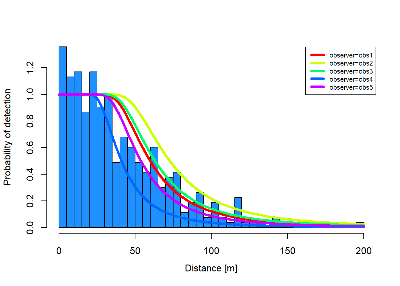
Figure 1: An estimated distance function relating Brewer’s sparrow observation distances (histogram bars) to individual observers (colored lines).
Note that Observer 4 had the smallest estimated ESW and Observer 2 the largest.
2 Average ESD and Confidence Interval
The Rdistancesummary() method prints average ESD (ESW in this case), along with minimum and maximum ESD. The ‘Average effective strip width (ESW)’ line in the summary output reports average ESW of 67.05, a minimum ESW among all covariate values (observers) of 47.67, and a maximum of 82.8. We know from the plot that the minimum applies to Observer 4, while the maximum applies to Observer 2.
2.1 Run Bootstraps
A confidence interval for average ESD can be calculated after bootstrap resampling of transects. Here, I run 500 bootstrap iterations.
Warning
Because ‘observer’ contains 5 levels (4 coefficients), bootstrap estimation is slow. 100 iterations took >20 minutes on an otherwise fast desktop. Planned updates to ‘Rdistance’ should speed calculation considerably. Until then, patience is required.
bsFit <- dfuncFit |> Rdistance::abundEstim(area = tenHectares , ci =0.95 , R =500 , plot.bs =FALSE , showProgress =TRUE)
Listing 2: Summary of the example distance function and abundance estimates after bootstrap resampling transects. Coefficient standard errors change and confidence intervals for density and abundance are reported.
summary(bsFit)
Call: dfuncEstim(data = sparrowDf, dist ~ observer +
   groupsize(groupsize), likelihood = "hazrate", w.hi = whi)
Coefficients:
              Estimate     SE         z           p(>|z|)
(Intercept)    3.97923469  0.1637128  24.3061986  1.685748e-130
observerobs2   0.19457534  0.1934083   1.0060342   3.143991e-01
observerobs3   0.05063578  0.2094501   0.2417558   8.089694e-01
observerobs4  -0.37709138  0.1668883  -2.2595439   2.384957e-02
observerobs5  -0.10615066  0.1688584  -0.6286371   5.295866e-01
k              3.25594658  0.5527929   5.8899938   3.862100e-09

Message: Success; Bootstrap SE's
Function: HAZRATE
Strip: 0 [m] to 200 [m]
Average effective strip width (ESW): 67.04909 [m] (range 47.674 [m] to 82.80148 [m])
Average probability of detection: 0.3352454 (range 0.23837 to 0.4140074)
Scaling: g(0 [m]) = 1
Log likelihood: -1642.054
AICc: 3296.35

     Surveyed Units: 36000 [m]
   Individuals seen: 372 in 354 groups
 Average group size: 1.050847
   Group size range: 1 to 3

Density in sampled area: 7.900855e-05 [1/m^2]
                 95% CI: 5.949629e-05 [1/m^2] to 0.0001071137 [1/m^2]

Abundance in 1e+05 [m^2] study area: 7.900855
                             95% CI: 5.949629 to 10.71137
Note
Rdistance versions >4.1.0 compute asymptotic standard errors for distance function coefficients until bootstrap sampling is complete. After bootstraps are run, Rdistance reports bootstrap standard errors for coefficients. Note the difference in coefficient standard errors between Listing 1 and Listing 2. In this case, bootstrap standard error estimates are on average 27% larger than the corresponding asymptotic estimates.
2.2 Inspect Bootstrap Object
Summaries of the bootstrap iterations appear in the $estimates component of the output object. These summaries include descriptive statistics, point estimates, and bias corrected bootstrap intervals for key study parameters.
as.data.frame(bsFit$estimates)
        id (Intercept) observerobs2 observerobs3 observerobs4 observerobs5
1 Original    3.979235    0.1945753   0.05063578   -0.3770914   -0.1061507
         k              density           density_lo           density_hi
1 3.255947 7.900855e-05 [1/m^2] 5.949629e-05 [1/m^2] 0.0001071137 [1/m^2]
  abundance abundance_lo abundance_hi avgEffDistance avgEffDistance_lo
1  7.900855     5.949629     10.71137   67.04909 [m]      54.35538 [m]
  avgEffDistance_hi nGroups nSeen avgGroupSize        area surveyedUnits
1      77.19479 [m]     354   372     1.050847 1e+05 [m^2]     36000 [m]
  propUnitSurveyed       w
1                1 200 [m]
All bootstrap iterations are stored in the output object’s $B component. The quantities that Rdistance computes and saves during bootstrap iterations are:
id = Bootstrap iteration ID
\(\beta\) = Coefficients (\(p\) columns)
density = Density of targets in sampled area
abundance = Abundance of targets on study area
nGroups = Number of groups seen
nSeen = Number of individuals seen (sum of groupsize over groups)
avgGroupSize = Average group size (nSeen / nGroups)
area = Study area size
surveyedUnits = Total length of transects sampled
propUnitSurveyed = Proportion of the default sampled area that was observed
w = Nominal maximum strip width or radial distance
avgEffDistance = Average effective sampling distance
In this tutorial, we are interested in the last column, avgEffDistance. Bias corrected bootstrap confidence intervals can be computed by the bcCI routine in Rdistance. bcCI requires the bootstrap values and the original point estimate.
Bias corrected intervals on average ESW are actually easier than that. Rdistance computes bias corrected intervals and stores them in the $estimates component.
# These should match the 'avgESW_estimate' in immediately prior code chunkbsFit$estimates[c("avgEffDistance", "avgEffDistance_lo", "avgEffDistance_hi")]
In this tutorial, the bias corrected and percentile confidence intervals are nearly identical. In general, I prefer bias corrected confidence intervals, unless the bootstrap distribution is very skewed. If the bootstrap distribution is very skewed, I prefer straight percentile intervals, unless the histogram shows significant bias. I realize this note is not helpful in practice when both bias and skewness are suspected; but, perhaps it is useful when only bias or skewness (but not both) are suspected.
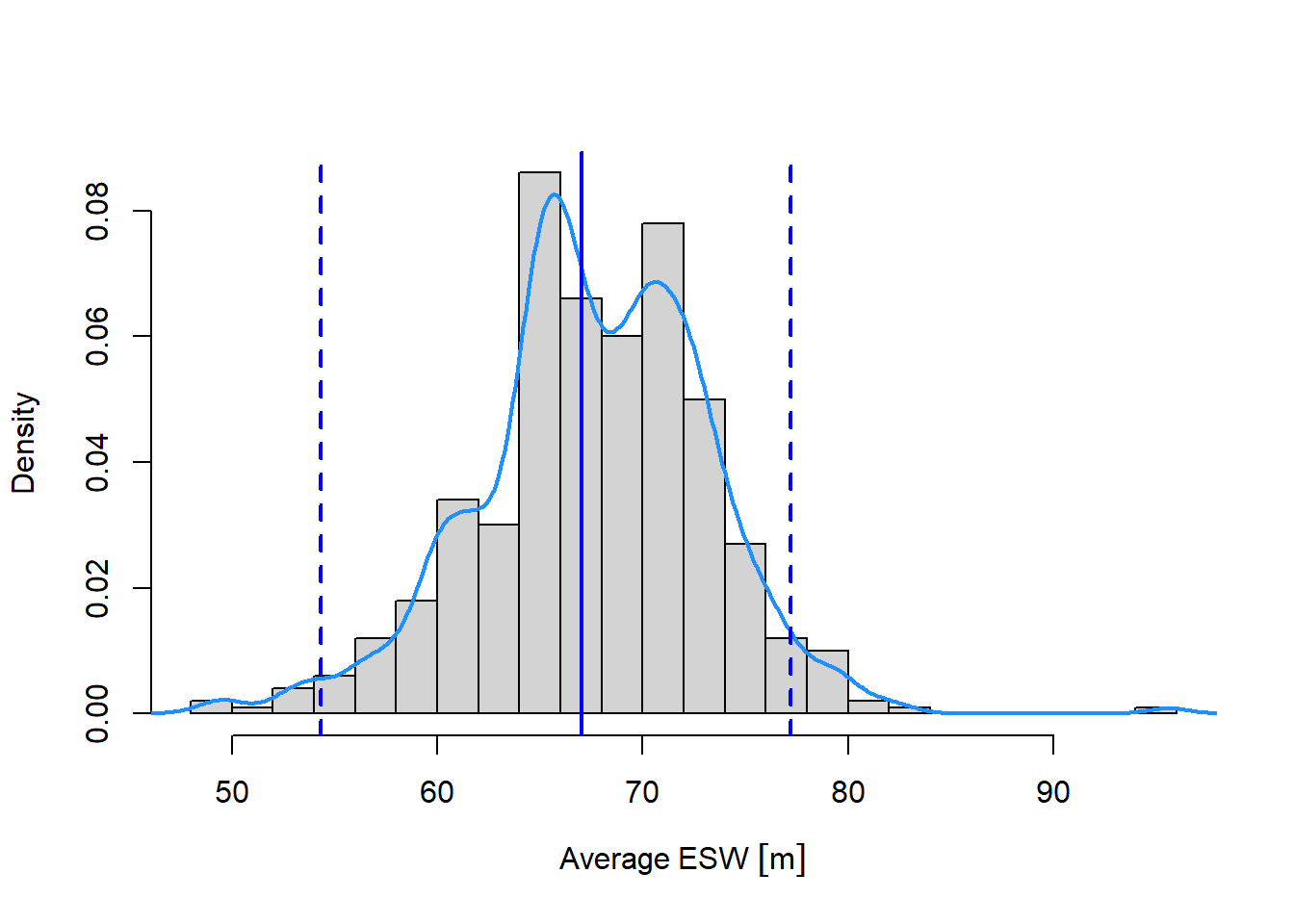
The bootstrap distribution of ESW can be visualized in many ways. The following basic plot method shows the average ESW histogram and confidence interval endpoints.
Figure 2: Bootstrap distribution of average ESW for Brewer’s sparrow (grey bars, light blue line) showing the point estimate of average ESW (vertical blue line) and 95% confidence interval endpoints (vertical dashed lines).
Final Notes
Caution
Estimates of average ESD are of general interest and can be used for study planning, etc. Average ESD cannot be used to compute density or abundance. While it might be tempting, you cannot compute abundance as follows:
# DO NOT DO THISn <-sum(unnest(sparrowDf)$groupsize, na.rm = T) # Number seenL <-sum(sparrowDf$length) # Total transect lengthA <- units::set_units(tenHectares, "m^2") # Study area size, in m^2wrongAbundance <- (A * n) / (2* avgESW_estimate[c(1,3,2)] * L)wrongAbundance
Density and abundance should be computed using the “Horvitz-Thompson” approach that inflates each observation by its probability of detection. The HT approach requires separate effective sampling distances for each observation. Observation-specific ESD then inflate observation-specific group sizes, and these inflated group sizes are summed. To illustrate on current data, the HT calculations first subset observations to those inside the nominal strip, then individual group sizes are inflated (divided by) individual ESD, and the result is summed.
# Horvitz-Thompson estimate of abundancesightingsInStrip <-unnest(sparrowDf) |> dplyr::filter( !is.na(groupsize) ) |># drop zero transects dplyr::filter( dist <= whi ) # drop obs outside stripn <- sightingsInStrip$groupsize # obs-specific groupsizes (no summing this time)esw <-ESW(dfuncFit, newdata = sightingsInStrip) # obs-specific ESDcorrectAbundance <- A *sum( n / (2* esw * L)) # inflate, then sumcorrectAbundance
7.900855 [1]
# compare to
bsFit$estimates$abundance
[1] 7.900855
Notes on L
Note 1: Total transect length (L in the above calculations) must include the ‘zero’ transect lengths. n and esw do not necessarily need to include ‘zero’ transects because n on ‘zero’ transects is zero.
Defn: ‘zero’ (or ‘blank’) transects are those without detections.
Note 2: L is constant during HT abundance calculations. If transect lengths vary, we do not inflate group sizes by (divide by) individual transect lengths. We ‘pool’ all strips from all transects and compute density on this aggregate area. To make this clear, it might be better to illustrate the equivalent HT calculations using ‘p’, the probability of detection, i.e.,
p <- esw / whi # probability of detecting each target (a vector)a <-2* whi * L # total (rectangular) area observed by all transects (a scalar)correctAbundance2 <- A *sum( n / p ) / a correctAbundance2
7.900855 [1]
The ‘pooled’ area (i.e., a <- 2*whi*L), is generally called the ‘observed area’, and we usually say things like, “Density on the observed area was…, while abundance on the study area was…”