The huber distance function was added to Rdistance as of version 4.4.0. This tutorial illustrates what it looks like and compares it to other distance functions.
Huber Definition
Rdistance’s huber likelihood is an inverted version of the Huber loss function (Huber loss)1, mixed with a uniform at the upper end. We added two parameters to the classic Huber loss function to make it appropriate to use as a distance function; hence, Rdistance’s huber likelihood contains three canonical parameters.
The huber distance function is a negative quadratic function from w.lo to its first parameter \(\theta_1\), linear between \(\theta_1\) and the sum of its first and second parameters (\(\theta_1 + \theta_2\)), and constant at a height of \(p\) after \(\theta_1 + \theta_2\). \(p\) is huber’s third parameter. In equation form, the huber likelihood is, \[
f(d|\theta_1,\theta_2, p) = \left(1 -
\frac{(1-p)h(d)}{m}\right) \,
I(0 \leq d \leq \Theta) \ + \ p \, I(\Theta < d \leq w)
\] where \(I\) is the regular indicator function, \(\Theta = \theta_1 + \theta_2\), \(w\) = w.hi - w.lo, \(m = \theta_1(\Theta - 0.5\theta_1)\), and \(h(d)\) is the Huber loss between 0 and \(\Theta\), i.e., \[
h(d) = 0.5d^2\, I(0 \leq d \leq \theta_1) \ + \
\theta_1(d - 0.5\theta_1)\, I(\theta_1 < d \leq \Theta).
\] Like other distance functions, Rdistance’s huber likelihood can vary with covariates. The huber likelihood is related to covariates through its first parameter, \(\theta_1\), i.e., \[
log(\theta_1) = \beta_0 + \beta_1x_1 + \ldots + \beta_qx_q.
\] The other two parameters, \(\theta_2\) and \(p\) are constant across covariate values. Technically, the parameter vector for the huber likelihood contains \([\beta_0, \beta_1, \ldots, \beta_q, \theta_2, p, \text{<exansion coefficients>}]\)
Huber Shape
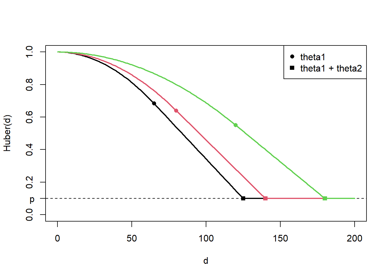
The Examples section of help(Rdistance::huber.like) contains a plot illustrating the huber likelihood’s shape. We replicate that plot here. The following code evaluates three huber distance functions from 0 to 200 at \(\theta_1\) values of 65, 80, and 120.
This code plots all three huber functions, showing parameter locations.
h <- y$L.unscaled # a matrixparams <- y$params # a matrixparams <- params[1,] # but params constant over rowsparams <-c(as.matrix(params)) # turn into vectornFuncs <-ncol(h)plot(range(d), range(h) , type ="n", xlab ="d", ylab ="Huber(d)", ylim =c(0,1))legend("topright" , legend =c("theta1", "theta1 + theta2") , pch =c(16,15) , col =1)abline(h = params[nFuncs +2], lty =2)axis(2, at = params[nFuncs +2], labels ="p", las =2)for(i in1:nFuncs){# Distance functionlines(d, h[,i], col = i, lwd=2)# Quadradic to linear transitions theta1 <-exp(params[i])points(theta1 , h[(theta1-0.1) < d & d < (theta1+0.01),i] , pch =16 , col = i )# Linear to constant transition Theta <- theta1 + params[nFuncs +1] # no link on theta2points(Theta , h[(Theta-0.1) < d & d < (Theta+0.1),i] , pch =15 , col = i )}
Figure 1: Three huber distance functions showing shape and location of the canonical parameters. The function is a negative quadratic between 0 and theta1 (dots), linear between theta1 and theta1+theta2 (squares), and constant at p beyond theta1+theta2.
Huber and Others
The Huber distance function is flexible and has several characteristics we want in distance functions. For example, the derivative of the Huber distance function is zero at zero, which means the function is technically horizontal at the x intercept (= distance 0). This characteristic matches the half normal, hazard rate, and oneStep distance functions. The Huber distance function has a ‘shoulder’ similar to the half normal function. Huber’s ‘shoulder’ is quadratic in shape, while the half normal’s is exponentially quadratic. Huber’s ‘shoulder’ does not (cannot) extend as far as the hazard rate function’s and this is an important difference. Perhaps Huber’s most useful characteristic is the uniform distribution mixed in to model large distances. This mixture process means that a ‘small trickle’ of large distance values do not cause instability, and right-truncating a small fraction is not necessary.
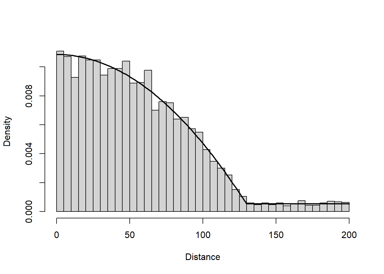
To illustrate shape among distance functions, we plot huber, triangle, oneStep, halfnorm, and hazrate distance functions on top of one another. To make this illustration meaninful, we fit these distance functions to the same simulated dataset. The next code chunk generates 5000 random distances from the Huber likelihood using the inverse-CDF method. we compute the Huber CDF by scaling the output of Rdistance::huber.cumFunc. In this example, we use Huber parameters \(\theta_1\) = 120, \(\theta_2\) = 10, and \(p\) = 0.05, and generate distance values between 0 and 200.
# Parameter valuesc(R = R, theta1 = theta1, theta2 = theta2, p = p, w = w)
      R  theta1  theta2       p       w
5000.00  120.00   10.00    0.05  200.00
Figure 2: 5000 random values drawn from the Huber distance likelihood. Black line is the true generating Huber distance likelihood with parameters 120, 10, and 0.05
Next, we fit distance functions to the simulated data. To do that in Rdistance, we create an ‘RdistDf’ data frame.
# Create the 'RdistDf'. Pretend only 1 transectdistDf <-data.frame(transect =1, distance =setUnits(rhuber, "m"))siteDf <-data.frame(transect =1, length =setUnits(1000, "m"))huberDf <-RdistDf(siteDf, distDf)huberDf
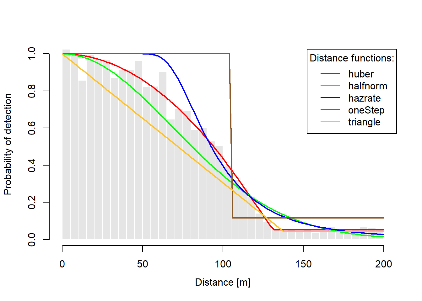
Figure 3: Shape and fit comparision of distance functions for the same data set.
Figure 3 shows that the huber function fits this fake dataset really well, which is good because we generated the data from a Huber likelihood. The AIC statistics and effective strip widths, sorted by AIC, appear in Table 1.
Table 1: AIC and ESW for the example distance functions.
Function
ESW
AIC
DeltaAIC
huber
92.45 [m]
49124.88
0.00
hazrate
100.99 [m]
49232.90
108.02
halfnorm
85.59 [m]
49332.02
207.13
oneStep
116.46 [m]
49606.73
481.84
The author notes that estimates of individual huber parameters are often different from their true values2, but that their sum usually well estimates the threshold (i.e., the discontinuity where the Huber meets the uniform). This makes sense because the transition from quadratic to linear at \(\theta_1\) is smooth3 and designed to be subtle. The discontinuity at \(\theta_1 + \theta_2\) is much less subtle and easier to estimate.
Here, estimates of the transition to linear (\(\hat{\theta}_1\)) and width of the linear part (\(\hat{\theta}_2\)) are relatively far from their generating values (Table 2). The discontinuity estimate (\(\hat{\theta}_1 + \hat{\theta}_2\)) is very close to the true value largely due to the enormous sample size.
Table 2: True and estimated parameters from the example data.
Parameter
True
Estimated
Theta1
120.00
110.776
Theta2
10.00
20.401
Theta1 + Theta2
130.00
131.178
p
0.05
0.052
Regarding shape differences, Figure 3 shows that the halfnorm has trouble fitting the steep decline in observations between approximately 75 and 125, while the hazrate has trouble fitting the gradual decline in observations between 0 and approximately 75. These two observations are not really fair because we generated data that explicitly do not fit the halfnorm and hazrate; but, these notes illustrate a couple key differences between huber and the others. The huber can fit relatively steep declines in observation numbers in the ‘mid range’ of the strip. The huber‘s ’shoulder’ (between 0 and approximately 75 here) is mid way between the halfnorm and hazrate ‘shoulders’. Finally, huber accommodates a ‘small trickle’ of really large observations. Further, huber provides an estimate of the location where the ‘small trickle’ starts (i.e., the discontinuity or \(\hat{\theta}_1 + \hat{\theta}_2\), here 131.2). The halfnorm and hazrate functions do not (cannot) fit a histogram containing a small but constant fraction of large values. The later two functions display marked lack-of-fit above approximately 115 and eventually decay to zero.
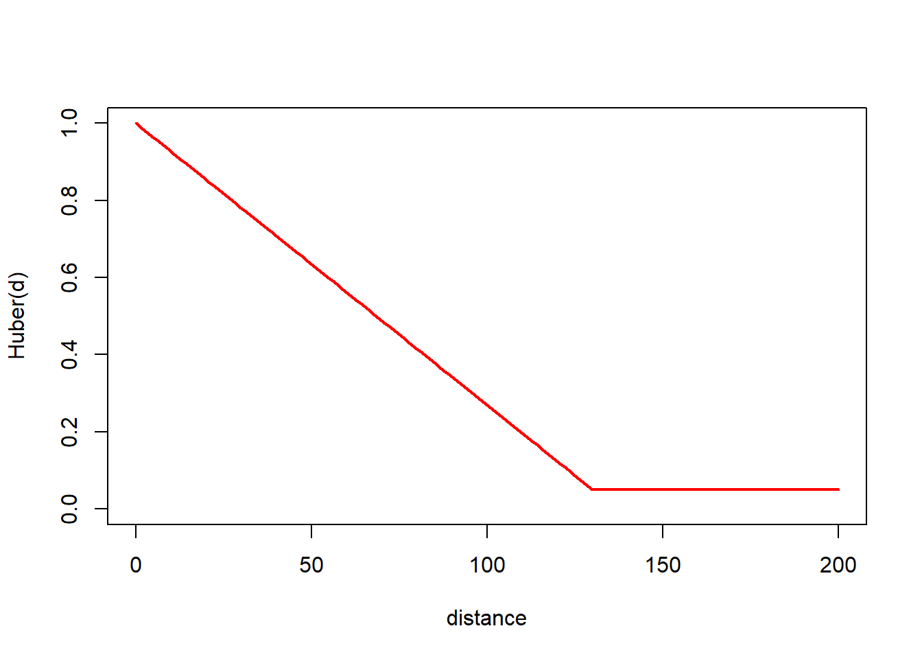
The huber likelihood can take on a wide variety of shapes depending. It’s first parameter, \(\theta_1\), must be greater than zero but has no maximum. When \(\theta_1\) is very small, the huber distance function converges to another distance function in Rdistance, the triangle function (Figure 4). As \(\theta_1\) grows large, the huber function converges to a uniform distribution on the strip 0 to \(w\) (Figure 5).
Figure 4: The huber likelihood with small \(\theta_1\) is the triangle likelihood. Here, \(\theta_1\) = 0.01, \(\theta_2\) = 130, and \(p\) = 0.05.
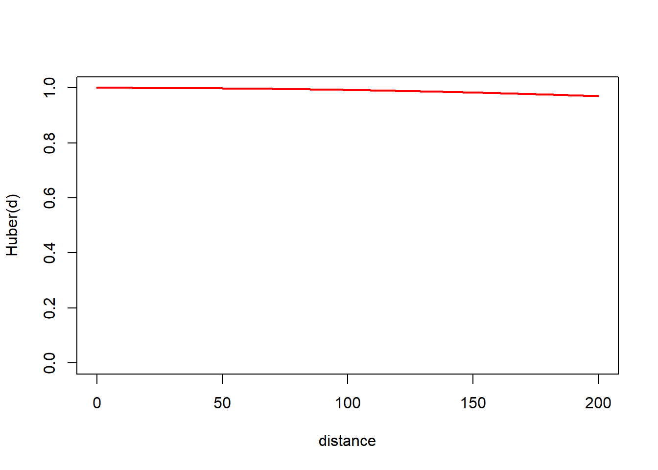
Figure 5: The huber likelihood with large \(\theta_1\) resembles a uniform distribution on [0,\(w\)]. Here, \(\theta_1\) = 1000, \(\theta_2\) = 130, and \(p\) = 0.05.
In conclusion, the huber distance function will be useful in situations where:
The left side (short distances) of the histogram shows slight declines. The ‘shoulder’ is not exactly flat, and could extent all the way to \(w\).
The decline in observations of middle-distances is fairly rapid.
A threshold exists past which only a few (large) values are observed.
Footnotes
The original paper is Huber, P. J. (1964). “Robust estimation of a location parameter”. Annals of Mathematical Statistics, 35 p. 73–101.↩︎
That is, have poor precision. Whether individual parameter estimates \(\hat{\theta}_1\) and \(\hat{\theta}_2\), and for that matter the threshold estimate \(\hat{\theta}_1+\hat{\theta}_2\), are unbiased remains to be determined.↩︎
Smooth means that the slope of two tangent lines, one on either side of but close to \(\theta_1\), are equal.↩︎