Huber Distance Function - With Covariates

This tutorial follows Huber Distance Function and illustrates fitting the huber function to factor covariates.

Huber Observations

For this tutorial, we generate distance observations from the Huber likelihood. We generated Huber observations using the inverse-CDF method in the previous Hubor tutorial. Here, we repeat the method and simulate separate Huber distributions in two habitat types, which we generically call ‘A’ and ‘B’. The following code generates 500 observations in habitat type ‘A’ from a Huber distribution with parameters (\(\theta_1\) = 50, \(\theta_2\) = 50, \(p\) = 0.05), and 500 observations in habitat type ‘B’ with parameters (\(\theta_1\) = 100, \(\theta_2\) = 50, \(p\) = 0.05). We pretend there is one 1000 [m] transect in each habitat type. We code habitat type as a two-level factor variable associated with transects.

# Simulation parameters:
R <- 500
theta1.1 <- 50
theta1.2 <- 100
theta2 <- 50
p <- 0.05
w <- 200

# Attache Rdistance
suppressPackageStartupMessages(library(Rdistance))

# Generate Huber values for habitat 'A' and 'B'
d <- 0:w
cdfA <- huber.cumFunc(d, theta1.1, theta2, p, w) / huber.cumFunc(w, theta1.1, theta2, p, w)
u <- runif(R)
dForA <- approx(cdfA, d, xout = u)$y

cdfB <- huber.cumFunc(d, theta1.2, theta2, p, w) / huber.cumFunc(w, theta1.2, theta2, p, w)
u <- runif(R)
dForB <- approx(cdfB, d, xout = u)$y

# Construct Rdist data frame with habitat factor
distDf <- data.frame(
    transect = rep(1:2, each = R)
  , distance = setUnits(c(dForA, dForB), "m")
  )
siteDf <- data.frame(
    transect = 1:2
  , habitat = factor(c("A", "B"))
  , length = setUnits(rep(1000,2), "m")
  )
huberDf <- RdistDf(siteDf, distDf)
huberDf

# A tibble: 2 × 4
# Rowwise:  transect
  transect         detections habitat length
     <int> <list<tibble[,1]>> <fct>      [m]
1        1          [500 × 1] A         1000
2        2          [500 × 1] B         1000

Fit the Huber Function

Rdistance relates the first huber parameter, \(\theta_1\), to covariates using function dfuncEstim. Maximization of the Huber likelihood takes a bit more time than others because of the extra parameters and employment of a non-gradient global maximization algorithm. On the author’s machine, Huber maximization in the next step completed in 4 to 5 seconds, while the halfnorm and hazrate completed in approximately 0.1 to 0.3 seconds.

fit <- huberDf |> 
  dfuncEstim(distance ~ habitat, likelihood = "huber")
summary(fit)

Call: dfuncEstim(data = huberDf, distance ~ habitat, likelihood =
   "huber")
Coefficients:
             Estimate  
(Intercept)   4.3378627
habitatB      0.4359016
theta2       26.9439138
p             0.0512715

Message: Success; SE's pending bootstrap
Function: HUBER  
Strip: 0 [m] to 197.514 [m] 
Average effective strip width (ESW): 87.26273 [m] (range 73.82413 [m] to 100.7013 [m]) 
Average probability of detection: 0.4418052 (range 0.3737665 to 0.5098439)
Scaling: g(0 [m]) = 1
Log likelihood: -4868.307 
AICc: 9744.653

Estimated parameters

The estimated parameters are,

ests <- data.frame(predict(fit, newdata = data.frame(habitat=c("A", "B")))) 
ests$Range <- ests[,"Theta1"] + ests[,"Theta2"]
ests

     Theta1   Theta2         p    Range
1  76.54376 26.94391 0.0512715 103.4877
2 118.36396 26.94391 0.0512715 145.3079

Here, the true parameter values in habitat type ‘A’ are (50, 50, 0.05) and their estimates are (76.54, 26.94, 0.05). Similarly, the true parameters in habitat ‘B’ are (100, 50, 0.05) and their estimates are (118.36, 26.94, 0.05). Estimates of the individual Huber parameters tend to have high variance and can be way off owing to the subtlety of the transition from quadratic to linear.

In contrast, the huber ‘range’¹ is well estimated. The true ranges in this example are 100 and 150 for habitat types ‘A’ and ‘B’, respectively. The estimated ranges are 103.49 and 145.31, respectively.

Plot

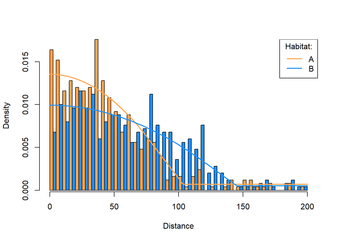
A nice visualization of the Huber function’s fit plots separate histograms for each habitat type with their associated distance function drawn over the top. The following plot shows the two histograms, one for habitat type ‘A’ and one for type ‘B’, side-by-side with the estimated density function in each type.² The following plot is a bit complicated to produce because we want side-by-side bars and that means everything needs to be scaled properly. We do this by calling hist to get bar heights, predict to get distance functions, and ESW to convert the distance functions into a density function.

barsA <- hist(dForA, breaks = seq(0,200,by=5), plot = FALSE)
barsB <- hist(dForB, breaks = seq(0,200,by=5), plot = FALSE)
bars <- rbind(barsA$density, barsB$density)
fittedDfuncs <- predict(fit
                 , newdata = data.frame(habitat = c("A","B"))
                 , distances = setUnits(0:200,"m")
                 , type = "dfunc")
scaleFactors <- ESW(fit, newdata = data.frame(habitat=c("A", "B")))
fittedDfuncs <- t( t(fittedDfuncs) / scaleFactors )

barplot(bars
        , beside = T
        , width = 2.5
        , xlim = c(0,200)
        , space=c(0,0)
        , col = c("tan1", "dodgerblue")
        , xlab = "Distance"
        , ylab = "Density"
        )
axis(1)

lines(attr(fittedDfuncs,"distances"), fittedDfuncs[,1], lwd=2, col="tan1")
lines(attr(fittedDfuncs,"distances"), fittedDfuncs[,2], lwd=2, col="dodgerblue")

legend("topright"
     , title = "Habitat:"
     , legend = c("A", "B")
     , lwd = 2
     , col = c("tan1", "dodgerblue")
     , lty = 1
     )

Figure 1: Histograms of simulated data in two habitat types, with huber density functions fitted to each.

Note

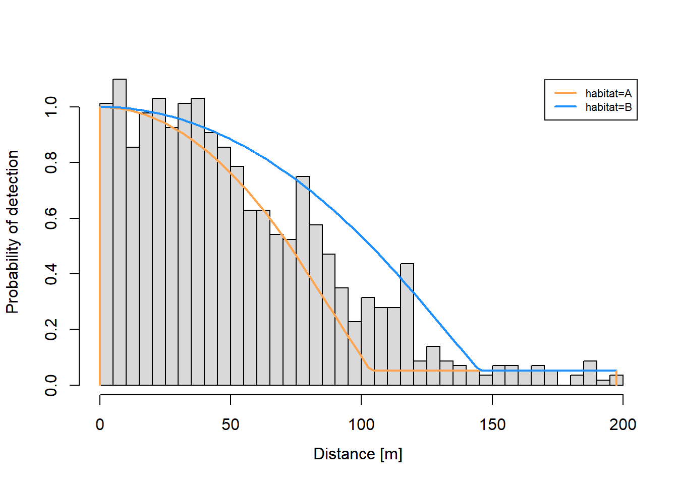
Figure 1 is the best kind of visualization for problems containing factors. The default Rdistance plot (Figure 2), is accurate but not great for visually assessing fit. Rdistance’s default plot does not distinguish factor levels in the bars and scaling of bars is for the overall problem not individual levels. These features obscure goodness of fit for individual factor levels.

plot(fit
     , newdata = data.frame(habitat = c("A", "B"))
     , nbins = seq(0,200,by=5)
     , col.dfunc = c("tan1", "dodgerblue"))

Figure 2: Rdistance’s default plot for the example. Bars are combined across habitat levels, scaling is not correct for individual factor levels, and hence fit is difficult to assess.

If this were a real problem, we would estimate abundance in the usual Rdistance way. We would estimate abundance by executing fit |> abundEstim(area=setUnits(X,"ha")), where X is study area size in hectares. Here, estimating abundance does not make sense because we generated distance observations, not densities, and we used only one transect in each habitat type.

Final Comments

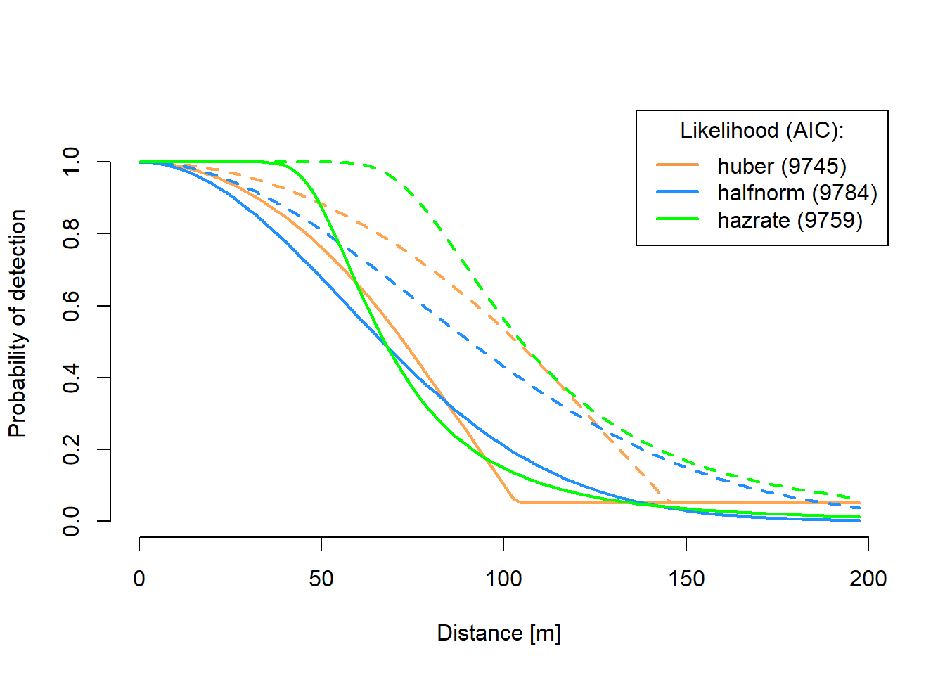
The huber likelihood differs from others in that its rate of decline in the ‘middle’ distances is steeper than the halfnorm and less than the hazrate, while its ‘shoulder’ is mid-way between the ‘shoulders’ of the halfnorm and hazrate (Figure 3).

Figure 3: The huber, halfnorm, and hazrate distance functions fitted to the same simulated data showing differences in ‘shoulders’ and rate of decline for ‘middle’ distances. Solid lines are for habitat type ‘A’. Dashed lines are for habitat type ‘B’.

Footnotes

1. Range of the huber likelihood is \(\theta_1 + \theta_2\).

2. We usually plot the distance function. The density function is the distance function scaled by effective strip width. We usually express this as \(f(x) = g(x)/\int g(x) dx\) where \(g(x)\) is the distance function with x intercept =1 and \(f(x)\) is the density function.